

What Is Multitask Learning? (Shared Backbone + Task Heads Explained)
Learn MTL using the x² and x³ example, including loss weighting and why tasks can dominate training.

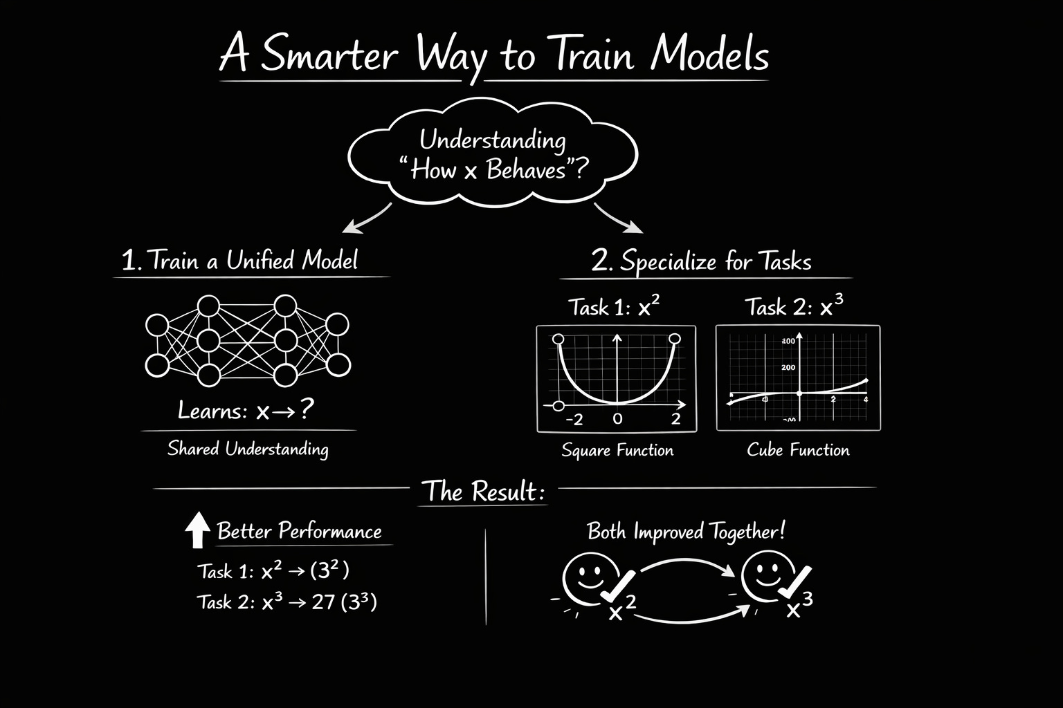
What if one neural network could learn two tasks at once like predicting x² and x³ from the same input? That tiny example captures the entire idea of multitask learning: one shared backbone, multiple task heads and better generalization.
Instead of training two separate models (one for x², one for x³), you train one model that learns a shared understanding of “how x behaves,” then specializes that knowledge for both tasks. Often, both tasks improve compared to training separately when the tasks are related and training is balanced.
Does it seem too good to be true? Let’s walk through it with a tiny example.
What is Multitask Learning?
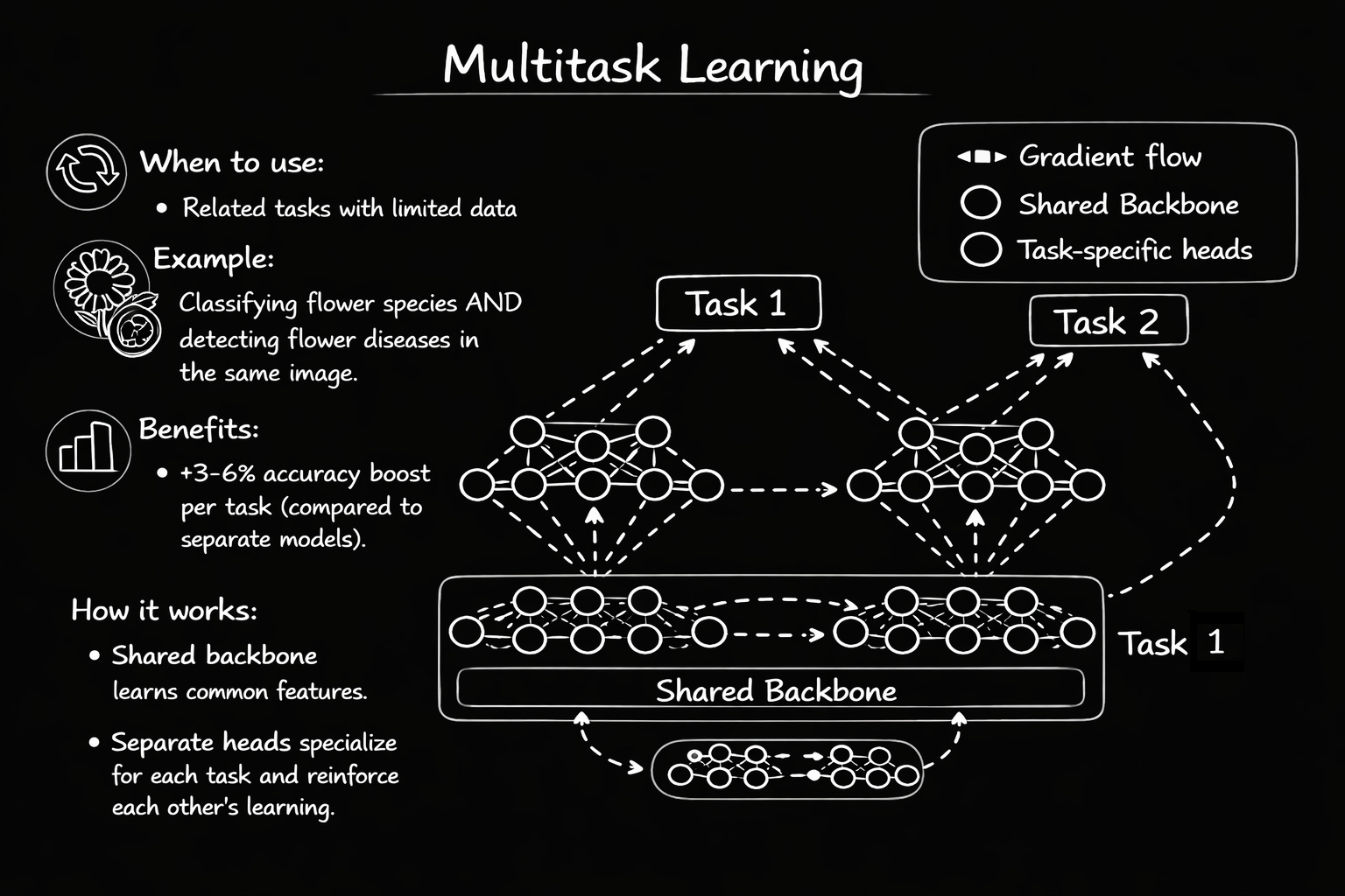
Multitask Learning (MTL) trains one neural network to solve multiple related tasks simultaneously.
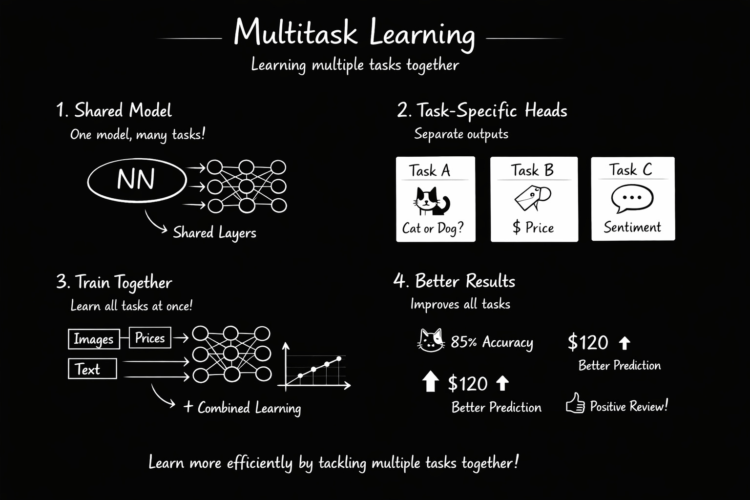
The Core Architecture
Every MTL model has two parts:
1. Shared Backbone Learns features that help all tasks. In medical imaging, it learns to recognize lung tissue, lesions, and anatomical structures. In NLP, it learns word meanings and sentence structure.
2. Task-Specific Heads Small, lightweight networks that take the shared features and turn them into task-specific predictions. One head might classify diseases, another might locate lesions, another might assess severity.
Piano and guitar analogy: Learning both instruments simultaneously develops general finger dexterity (shared skill), then each hand specializes for its instrument (task-specific skill). The shared learning makes you better at both faster than learning them completely separately.
Why does this actually work better?
Here’s what seems counterintuitive at first: learning multiple tasks together often makes each individual task perform better than if you trained them separately. How?
1. It prevents overfitting
A single-task model can memorize noise. For example, if you’re training on chest X-rays and most diseased patients happen to be photographed at a certain angle, the model might learn “this angle = disease” instead of actual pathology.
But in MTL, the backbone must satisfy multiple tasks at once. It can’t just memorize the camera angle because that doesn’t help with localization or severity scoring. Only real disease patterns help all tasks. This forces the model to learn genuine, generalizable features.
In practice, this is one of the biggest reasons MTL helps
2. Tasks help each other
Learning to locate a lesion teaches the model about disease characteristics, which helps with diagnosis. Learning severity teaches about disease progression, which helps both diagnosis and localization.
It’s learning synergy. Features learned for Task A improve Task B, and vice versa. Both tasks end up better than if trained alone.
3. One forward pass, multiple outputs
Instead of running an image through three separate models, you run it through one backbone, then branch to three lightweight heads. Faster inference, less memory, lower compute costs.
x² and x³
Two Ways to Build MTL Models
There are actually two architectural approaches to multitask learning.
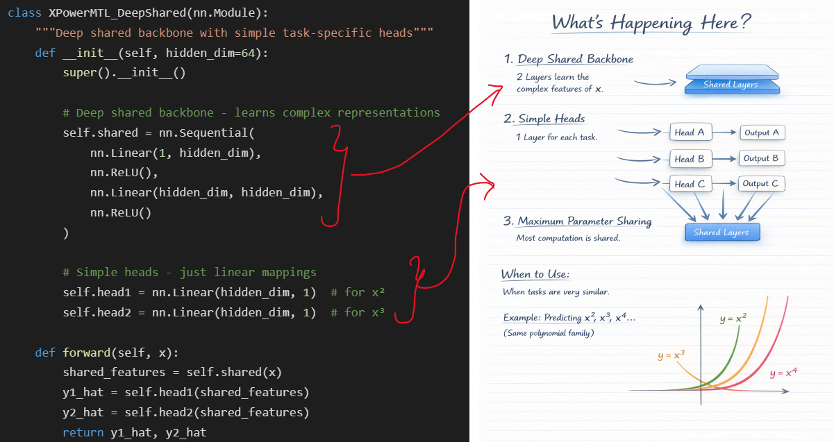
Approach 1: Deep Shared Backbone + Simple Heads
Philosophy: Heavy feature extraction in shared layers, lightweight heads
Use when: Tasks are very related and share most of their structure
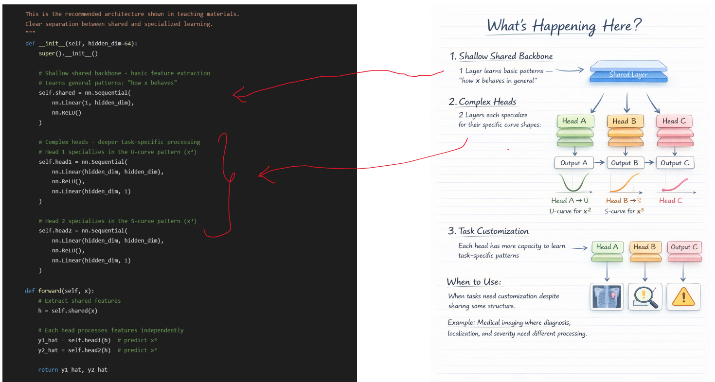
Approach 2: Shallow Shared Backbone + Complex Heads
Philosophy: Basic shared features, specialized task-specific processing
Use when: Tasks need customization and specialized processing
Understanding the Architecture
Part 1: The Shared Backbone (self.shared)
We have some fully connected layers in self.shared → These are the shared layers.
In Approach 2, the shared backbone is intentionally shallow:
INPUT: x = -2.0 (shape: [1, 1])
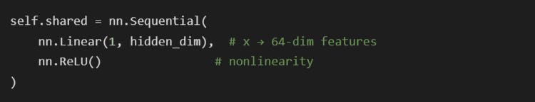
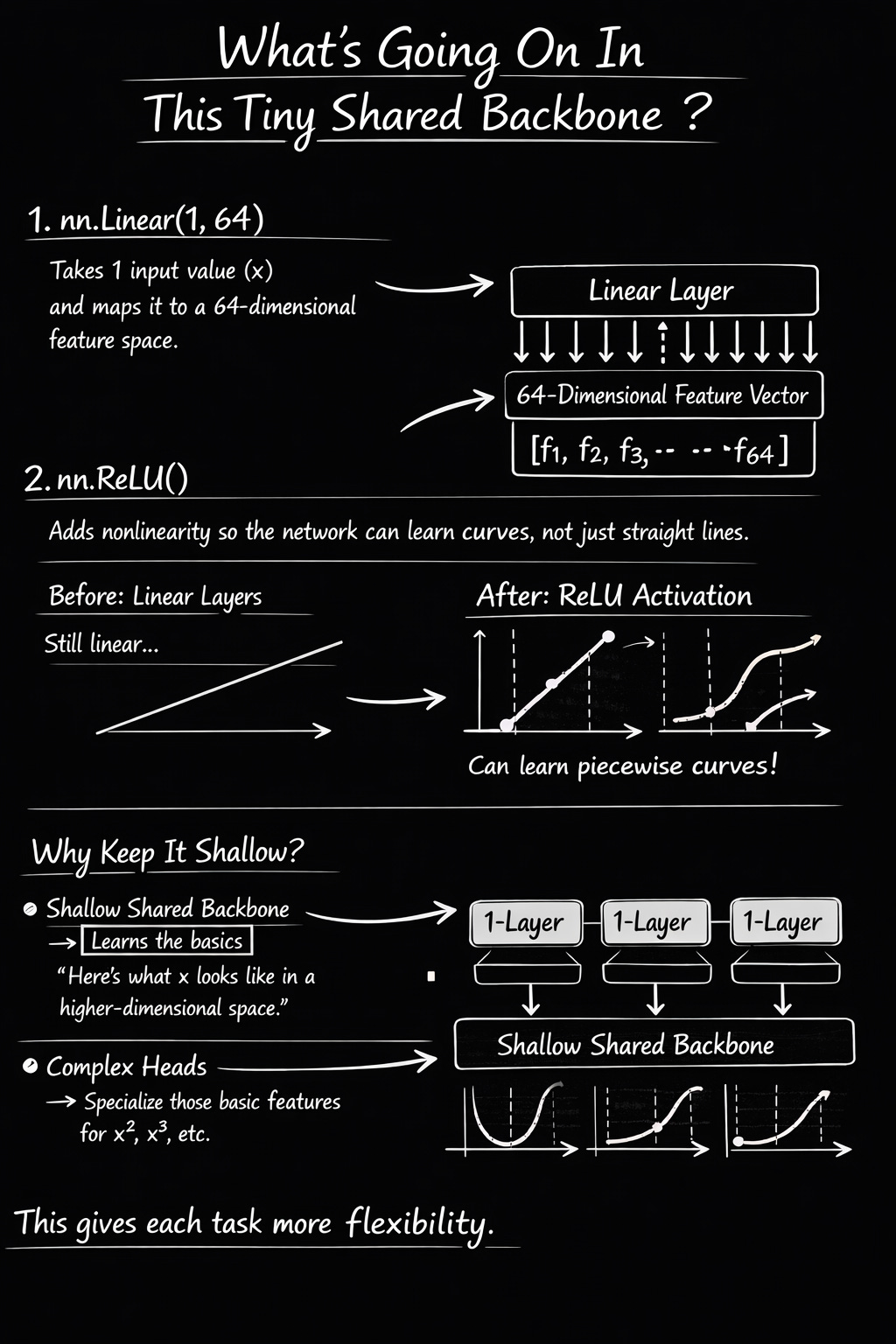
Layer 1: nn.Linear(1, 64)
What it does: Multiplies x by 64 different weight values, adds 64 bias values
Mathematically: h₁ = W₁·x + b₁, where W₁ is [64×1] and b₁ is [64]
Output: 64 numbers (one for each “dimension”)
Example output: [0.23, -1.45, 0.89, -0.12, …, 0.67] (64 values total)
This layer asks 64 different “questions” about x. Each weight learns to detect a different pattern. For example, one weight might learn “is x negative?”, another “is x large?”, another “is x near zero?”. The 64 numbers capture different aspects of x.
Layer 2: nn.ReLU()
What it does: ReLU(x) = max(0, x) — replaces all negative numbers with zero
Mathematically: h₂ᵢ = max(0, h₁ᵢ) for each of the 64 values
Output: [0.23, 0, 0.89, 0, …, 0.67] — same 64 values but negatives zeroed out
Intuition: ReLU introduces nonlinearity. Without it, stacking linear layers would just be one big linear transformation. ReLU lets the network learn curves, bends, and complex patterns. The “zeroing out” creates a decision: “this feature is relevant” (positive) or “ignore this feature” (zero).
Final Output: h (shared features)
Shape: [1, 64] — a 64-dimensional vector
Meaning: This is a “rich representation” of x in a higher-dimensional space
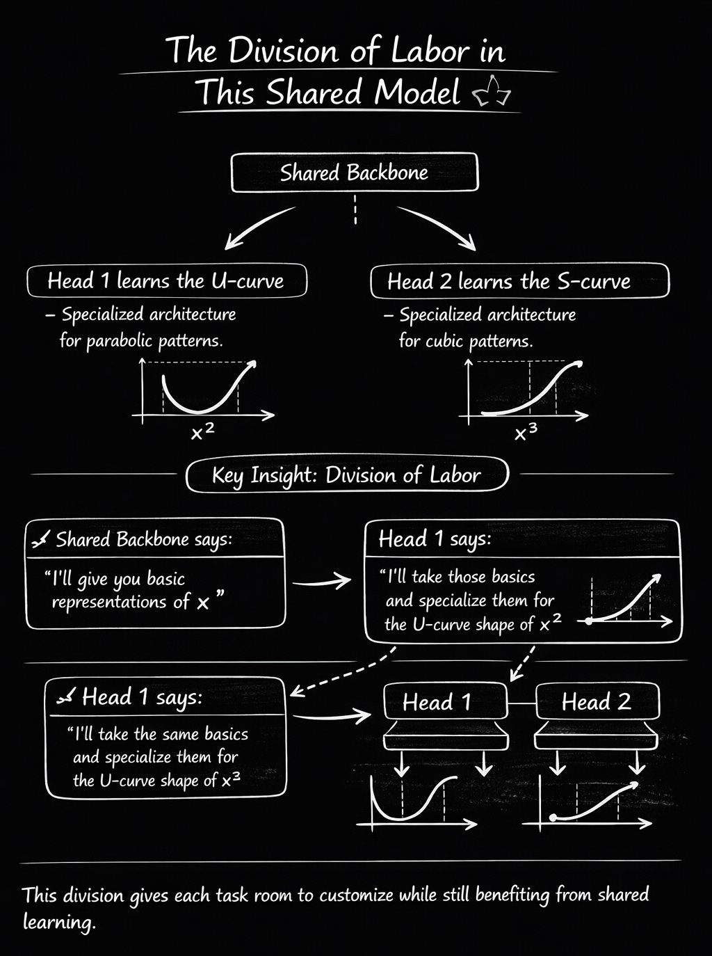
Key point: h captures GENERAL patterns about x that will help BOTH tasks
What did the shared backbone learn?
It learned to transform a single number (x) into a 64-dimensional representation (h) that captures useful patterns. Think of it like translating a sentence into 64 semantic features: “sentiment”, “formality”, “urgency”, etc. Here, we’re translating x into features like “magnitude”, “sign”, “proximity to zero”, “squared value”, etc.
Training with Weighted Losses
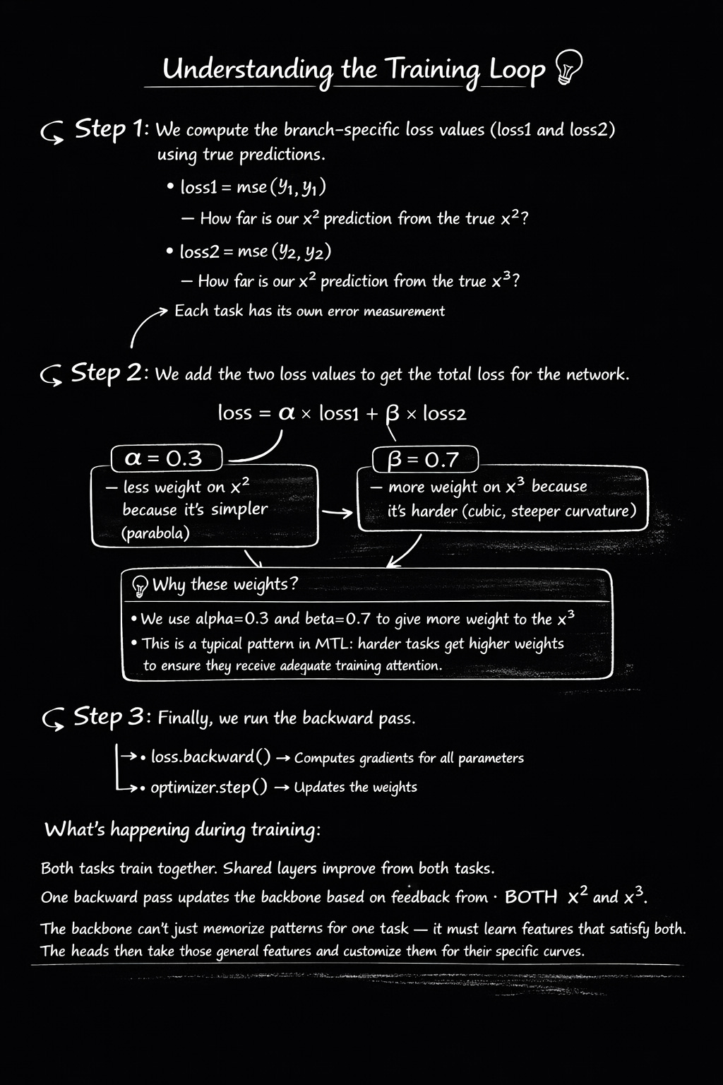
Why Weighted Losses Matter: A Numerical Example
Training Results
With this, we have trained our MTL model. As training progresses:
Loss1 decreases → model gets better at predicting x² (U-curve)
Loss2 decreases → model gets better at predicting x³ (S-curve)
Total loss decreases → overall performance improves
Both heads learn their specialized patterns
Shared backbone learns general features that help both
We get a decreasing loss, which depicts that the model is being trained. And that’s how we train an MTL model.
You can extend the same idea to build any MTL model of your choice — just replace x² and x³ with your actual tasks (disease classification, object detection, sentiment analysis, etc.), and follow the same pattern: shared backbone + task heads + weighted combined loss.
Multitask learning is simply one backbone learning general features, while multiple heads learn task-specific outputs all trained together using a weighted combined loss.
When and Why MTL Fails
MTL is not magic. It clearly backfires in some circumstances. Let me tell you the truth about the modes of failure.
Failure 1: There is no helpful structure among the tasks.
A poor example would be to train a single model to forecast weather and house prices.
No meaningful shared representation, different underlying processes (real estate markets vs. atmospheric physics), and different inputs (property features vs. meteorological data).
The model becomes confused if you make them share a backbone. It looks for features that fulfill both tasks, but none exist. Usually, both tasks perform worse.
Fix: Avoid using MTL. Train distinct models.
Failure #2: Training is dominated by one task.
The issue is that only 10% of your training data is for Task B, while 90% is for Task A.
The model will optimize primarily for Task A because it receives significantly more gradient updates, even if the tasks are related. Because Task B is “starved,” it may perform worse than a single-task model that was trained using just 10% of the data.
Adding an additional task actually degrades performance, which is one of the most frequent causes of negative transfer.
Fix:
Use loss weighting to upweight the minority task
Or use task-balanced sampling
If it still doesn’t improve, split into separate models
Rule of thumb
Always compare each task’s MTL performance against a strong single-task baseline.
If a task is worse in MTL → negative transfer is happening. Rebalance or split.
Now you understand MTL in the simplest possible way.
But the real fun starts when we take this exact idea and apply it to a real dataset.
For the Part 2 Follow me on Tina Sharma - Medium
Part 2: Multitask Learning on Medical Data
In Part 2 published on Towards AI (Medium), I take multitask learning from the toy example to a real medical dataset: NIH ChestX-ray14 (112,120 X-rays).
You’ll see how I:
convert labels into multi-hot vectors (14 diseases)
add a second task for abnormal vs normal
handle class imbalance using sample weights
build a fast tf.data pipeline
train EfficientNetB0 using a warmup + fine-tune strategy
reach ~0.71 AUC on abnormal detection (educational example)
If you want to reproduce this experiment, I’ve uploaded the full notebook here:
🔗 GitHub Repo: https://github.com/itinasharma/DeepLearning/blob/ae521205988629087963369e203ef023b7746dcd/mtl_x2_x3_pytorch_py.ipynb